
A gentle introduction to big O notation
23 Sep 2019 - John
In my previous post, I explained how to solve an algorithm exercise and analyzed its big O efficiency. However, someone pointed out to me that the post assumes the reader is familiar with big O notation to begin with, and that I should at least clarify how it works.
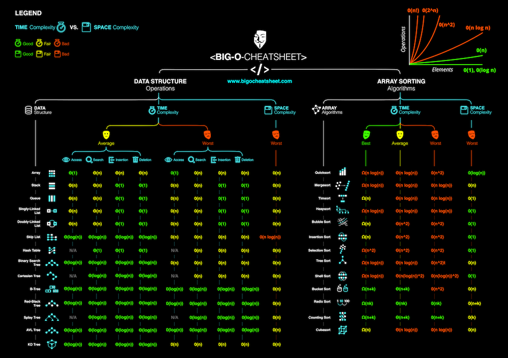
Credit: Big O cheat sheet
What is Big O notation?
Big O notation is a simplified way to measure an algorithm efficiency which is measured in two ways: space complexity and time complexity. We notate it by using the letter O, which stands for Order of, as in magnitude, and then use a denominator to express the complexity.
Space complexity
Space complexity analyses the resources your solution takes in the form of memory usage. For example, every time you assign a variable, it occupies a portion of your RAM, and of course, the more memory your solution uses, the less efficient it is.
Time complexity
While space complexity has to do with storage, time complexity is all about how long it takes your solution to execute.
Which one is more important?
While it is important to keep both in mind, time complexity takes the cake, so it will be the focus of this post. It’s generally accepted that the time it takes to run a program is more expensive than the space it takes in your computer. For example, a function that is BIG but fast will always be preferred over one that is small but it hits your cpu so hard that you can hear the fans kicking in: it’s even incurring in increased energy expenditure!
Getting started
To express the performance of an algorithm, you just have to write an O and then add a value, which depending on the case, can be any of the following:
O(log n): Regarded as logarithmic time. They start pretty fast, and their efficiency decreases very little as our data set gets larger:
for(let i = 0; i < n; i*2){
  console.log(i);
}
In this example, our counting variable i doesn’t go through the loop by incrementing the count one by one, but does so by multiplying the count until it reaches its target.
O(1): Known as constant time. These are simple statements like assigning a value or adding an element to an array:
let myArray = [1, 2, 3, 4]; // no looping, no iterating.
myArray.push(5); // just adding to an array.
The main takeaway with constant time is that it doesn’t matter what our input is, the operation is always going to take the same amount of time.
O(n): Also known as linear time. Loops will go to the full extent of our input and the execution time will increase as our input gets bigger:
let myVar = 10;
myFunction = (howManyTimes) => {
 for(let i = 0; i < howManyTimes; i++) {
   // do some stuff
 }
}
myfunction(myVar);
The most important thing to consider with O(n) is that the loop will always execute to the full size of our input. In this example, n is howManyTimes and the execution time will increase as we call the function with bigger numbers.
O(n²): Regarded as quadratic time. For every iteration of your n-based loop, there is going to be another loop executed. In plain words, this means loops within loops:
let myVar = 10;
myFunction = (howManyTimes) => {
  for(i=0; i < howManyTimes; i++) {
    for(j = 0; j < i; j++) {
     // Do some stuff
   }
  }
}
myFunction(myVar);
So when we call this function with an input of 10, we have a loop that will execute 10 times, but for each of those iterations, we have a loope that is going to run 10 other times, which effectively means it will run 10² = 100 times.
Does it mean I have to always shoot for n(1)?
Absolutely not. Different data structures have different methods of having operations performed to them so you need to get acquainted with what you can achieve with every data structure.
Further reading:
- Big O cheat sheet: Nice graph to check the complexity of your data types.
- Get ready for your coding interview (paid course): A paid, but great course in solving algorithms in Python.
- Big O cheat sheet: Another cheat sheet for Big O.